Gridded Wind Farm on a Rectangular Domain
This demonstration will show how to set up a 2D rectangular mesh with a wind farm consisting of a 36 turbines laid out in a 6x6 grid. This demo is associated with two files:
- Parameter File:
params.yaml- Driver File:
2D_Grid_driver.py
Setting up the parameters:
To write a WindSE driver script, we first need to define the parameters. This must be completed before building any WindSE objects. There are two way to define the parameters:
- Loading a parameters yaml file
- Manually creating the parameter dictionary directly in the driver.
Both methods will be discussed below and demonstrated in the next section.
The parameter file:
First we will discuss the parameters file method. The parameter file is the main way to customize a simulation. The driver file uses the options specified in the parameters file to run the simulation. Ideally, multiple simulations can use a single driver file and multiple parameter files.
The parameter file is formated as a yaml structure and requires pyyaml to be read. The driver file is written in python.
The parameter file is broken up into several sections: general, domain, boundaries, and wind_farm, etc.
The full parameter file can be found here: params.yaml and more information can be found here: Parameter File Explained.
Manual parameter dictionary:
The manual method involve creating a blank nested dictionary and populating it with
the parameters needed for the simulation. The windse_driver.driver_functions.BlankParameters()
will create the blank nested dictionary for you.
Creating the driver code:
The full driver file can be found here: 2D_Grid_driver.py First,
we start off with the import statements:
import windse
import windse_driver.driver_functions as df
Next, we need to set up the parameters. If we want to load them from a yaml file we would run:
# windse.initialize("params.yaml")
# params = windse.windse_parameters
However, in this demo, we will define the parameters manually. Start by creating a blank parameters object:
params = df.BlankParameters()
Next, populate the general options:
params["general"]["name"]        = "2D_driver"
params["general"]["output"]      = ["mesh","initial_guess","turbine_force","solution"]
params["general"]["output_type"] = "xdmf"
Then, the wind farm options:
params["wind_farm"]["type"]      = "grid"
params["wind_farm"]["grid_rows"] = 6
params["wind_farm"]["grid_cols"] = 6
params["wind_farm"]["ex_x"]      = [-1800,1800]
params["wind_farm"]["ex_y"]      = [-1800,1800]
params["wind_farm"]["HH"]        = 90
params["wind_farm"]["RD"]        = 126
params["wind_farm"]["thickness"] = 10
params["wind_farm"]["yaw"]       = 0
params["wind_farm"]["axial"]     = 0.33
and the domain options:
params["domain"]["type"]    = "rectangle"
params["domain"]["x_range"] = [-2500, 2500]
params["domain"]["y_range"] = [-2500, 2500]
params["domain"]["nx"]      = 50
params["domain"]["ny"]      = 50
Lastly, we just need to define the type of boundary conditons, function space, problem formulation and solver we want:
params["boundary_conditions"]["vel_profile"] = "uniform"
params["function_space"]["type"] = "taylor_hood"
params["problem"]["type"]        = "taylor_hood"
params["solver"]["type"]         = "steady"
Now that the dictionary is set up, we need to initialize WindSE:
params = df.Initialize(params)
That was basically the hard part. Now with just a few more commands, our simulation will be running. First we need to build the domain and wind farm objects:
dom, farm = df.BuildDomain(params)
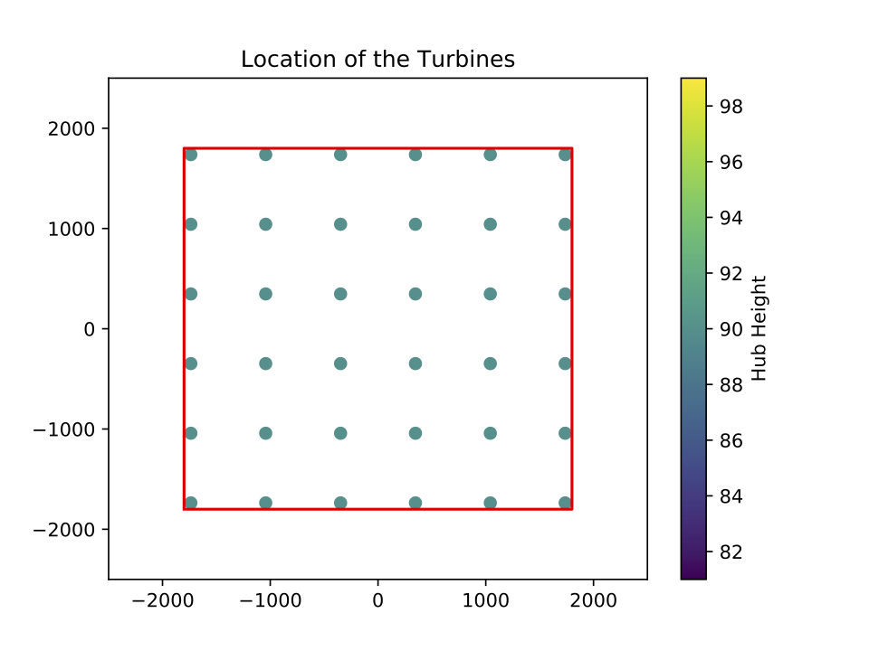
We can inspect the wind farm by running:
farm.Plot(True)
This results in a wind farm that looks like this:
Alternatively, we could have use False to generate and save the plot,
but not display it. This is useful for running batch test or on a HPC. We
could also manually save the mesh using dom.Save(), but since we
specified the mesh as an output in the parameters file, this will be done
automatically when we solve.
Next, we need to setup the simulation problem:
problem = df.BuildProblem(params,dom,farm)
For this problem we are going to use Taylor-Hood elements, which are comprised of 2nd order Lagrange elements for velocity and 1st order elements for pressure.
The last step is to build the solver:
solver = df.BuildSolver(params,problem)
This problem has uniform inflow from the west. The east boundary is our outflow and has a no-stress boundary condition.
Finally, it’s time to solve:
solver.Solve()
Running solver.Solve() will save all the inputs according to the
parameters file, solve the problem, and save the solution. If everything
went smoothly, the solution for wind speed should be:
